Frequency-independent solvers for oscillatory ODEs
Contents
- Introduction
oscode- fixed orderriccati- arbitrarily high order
1. Introduction
The methods described here were developed to solve second order, linear, homogeneous ODEs, i.e. those of the form \[\label{eq:osc} u’’ + 2\gamma(t)u’(t) + \omega^2(t)u(t) = 0, \quad t \in [t_0, t_1]. \] I generally work with initial value problems (IVPs) with initial conditions \[ u(t_0) = u_0, \quad u’(t_0) = u’_0, \] but the methods may be used to solve boundary value problems (BVPs) as well. I assume that $\omega(t)$ and $\gamma(t)$ are real-valued functions and $\omega(t) > 0$, but $u$ may be complex. This equation describes a generalized harmonic oscillator with time-dependent frequency $\omega(t)$ and friction term $\gamma(t)$. Depending on the magnitude of $\omega$ and $\gamma$, the solution oscillates rapidly or varies smoothly, sometimes switching back-and-forth between the two behaviors within the solution range $[t_0, t_1]$. For example, the analytic solution of \[\label{eq:burst} u’’ + \frac{100}{(1+t^2)^2}u(t) = 0, \quad t \in [t_0, t_1] \] undergoes a burst of oscillations around $t = 0$, as plotted below:

If one were to solve (\ref{eq:burst}) with any polynomial-based numerical method, (e.g. Runge–Kutta, linear multistep, spectral, simplectic integrators), the method would need to use a few discretization nodes per wavelength of oscillations, meaning that its computational effort would scale as $\mathcal{O}(\omega)$.
This is prohibitively slow at large $\omega$! What to do? The general strategy behind my solvers is:
- Use a more suitable basis. Both methods described below use asymptotic expansions designed for oscillatory functions to approximate $u(t)$ in regions where it is highly oscillatory, which allow for much larger stepsizes for the same number of discretization nodes (function evaluations/computational effort) than a polynomial approximation. These asymptotic expansions, however, only yield good approximations of $u$ if $\omega$, $\gamma$ are sufficiently smooth and $\omega$ is large. Therefore,
- Switch bases depending on how $u$ behaves. My methods use the asymptotic expansions when $\omega$ is sufficiently large, but automatically switch over to a polynomial-based solver when $u$ is not so oscillatory.
- Adapt. Update the stepsize/discretization length to keep the local error estimate below some user-defined tolerance.
Why should one care? Equations like (\ref{eq:osc}) are ubiquitous in physics and mathematics, and at the time of writing the papers listed below, no numerical method was able to deal with the solution exhibiting both highly oscillatory and nonoscillatory within the $t$-range of interest. I developed these solvers for use in primordial cosmology, but they found applications in fluid dynamics, astroparticle physics, quantum mechanics, and special function evaluation.
2. oscode - fast numerical solution of oscillatory ordinary differential equations
- developed in collaboration with Will Handley, Mike Hobson, and Anthony Lasenby (University of Cambridge, UK)
- paper DOI arXiv
- slides from a recent talk
- video summary
- open-source code (in C++ and Python) GitHub and its documentation
oscode switches between a 4th order Runge–Kutta method and a time-stepper
based on the Wentzel–Kramers–Brillouin expansion (abbreviated WKB, with a
fixed number of terms retained in the expansion) to advance the solution. At
this order, the method is most efficient if the required (relative) accuracy is
4-6 digits.
The WKB expansion is widely used in quantum mechanics to approximate steady-state wavefunctions in 1D potential wells, but has largely been applied analytically (“by hand”). This works fine if it only needs to be done once, but if an oscillatory ODE needs to be solved repeatedly with different coefficients, it quickly becomes unfeasible.
In cosmological inference, this is exactly what happens. In a Markov-chain Monte Carlo run, each point in parameter space defines a different family of ODEs, which need to be solved in order to compute a quantity called the primordial power spectrum. The ODE, called the Mukhanov–Sasaki equation, controls the evolution of quantum-scale perturbations during cosmic inflation. We later observe these fluctuations as anisotropies in the Cosmic Microwave Backgound (CMB), from which we can therefore make inference about the overall structure and evolution of the Universe. In a typical MCMC run (provided the primordial power spectrum needs to be evaluated numerically), $10^5$-$10^6$ spectra are calculated, which means around $10^8$-$10^9$ oscillatory ODE solves. Each oscillatory ODE solve can therefore at most take around a millisecond.
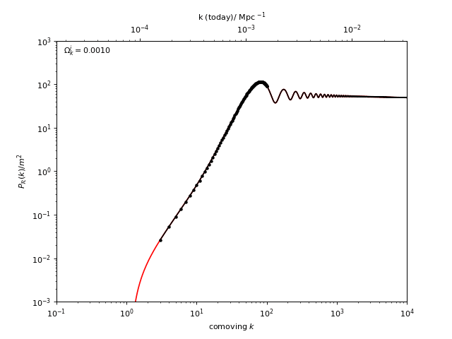
With oscode this is possible: the primordial spectra below
belong to closed universes with increasing initial curvature - it would take
$\geq $ 30 minutes to compute one of these on my laptop with a Runge–Kutta method from scipy, and
takes about 1 s with oscode at the same tolerance.
More uses of oscode in math and physics:
- Cosmology of closed universes:
- On physical optics approximation of stratified shear flows with eddy viscosity arXiv
- Some fast solvers for the 1D stationary Schroedinger equation that follow a similar strategy, but are higher order, have been developed, e.g. arXiv
3. riccati: arbitrarily high-order solver for oscillatory ODEs
- work with Alex Barnett (Flatiron Institute)
- paper arXiv
- slides
- code repository GitHub and documentation
riccati builds on some of the ideas behind oscode, but the underlying
methods it chooses between (in oscillatory/nonoscillatory regions of the
solution) are different and, importantly, arbitrarily high order. This
ensures that riccati remains efficient even if 10-12 digits of accuracy are
required.
In oscillatory regions, we introduced a novel asymptotic expansion, which we named adaptive Riccati defect correction (ARDC). Its main advantage lies with its simplicity: not only can the expansion be computed recursively, the recursion formula only depends on the previous term (as opposed to all previous terms for the WKB approximation). It can be computed numerically, without writing out analytic formulae. This also allowed us to prove that the expansion reduces the residual (~error) geometrically for the first $\mathcal{O}(\omega)$ iterations, and put an upper bound on its error.
In regions where the solution is slowly varying, riccati switches to
spectral collocation based on Chebyshev polynomials. The degree of
polynomials used can be set by the user.
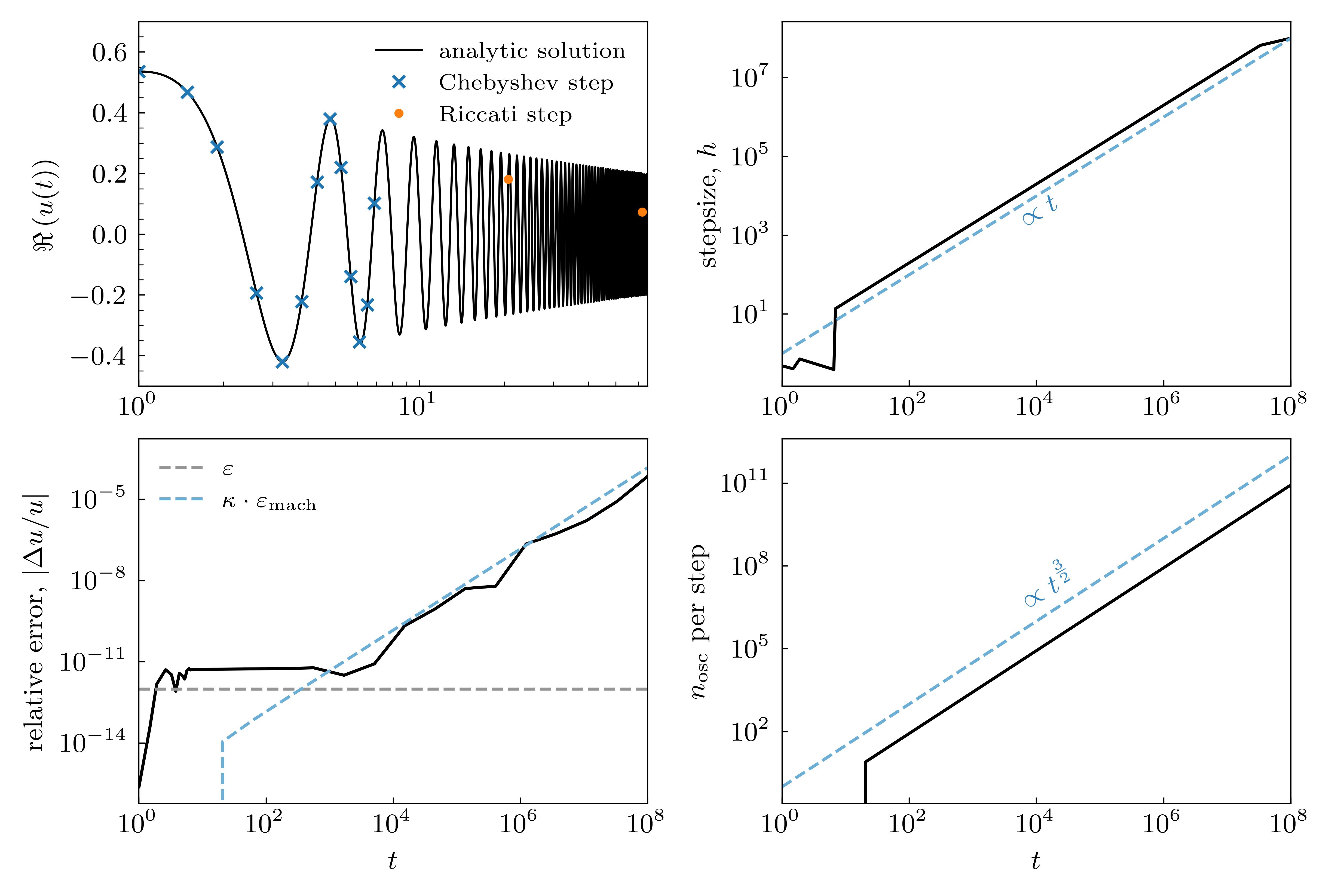
Below is the numerical solution of the Airy equation, $u’’ + ut = 0$ from $t = 1$ to $t = 10^8$, computed by riccati. I asked for 12 digits of accuracy, which it achieves initially, until the condition number of the problem increases and no longer allows this. The blue dashed line indicates an estimate of the best accuracy allowed by the conditioning of the problem – this is achieved.